One very painful aspect of searching for a job as an experienced software engineer is preparing for leetcode datastructures algorithms problems again from scratch. Your 🧠 brain cache can only hold so much information at a particular point of time and if you’re actually doing work at your job you’ll definitely forget solving DSA problems quickly. The keyword here is quickly because you’re expected to solve within a 30 minute or 45 minute time window. That’s why you need to learn to do pattern matching quickly.
This article refers heavily from these two links : Leetcode Cheatsheet and ByteByteGo Interview Patterns
Big O Complexity Chart

Remember that n! > 2^n because values > 2 get multiplied n times !
Problem Patterns
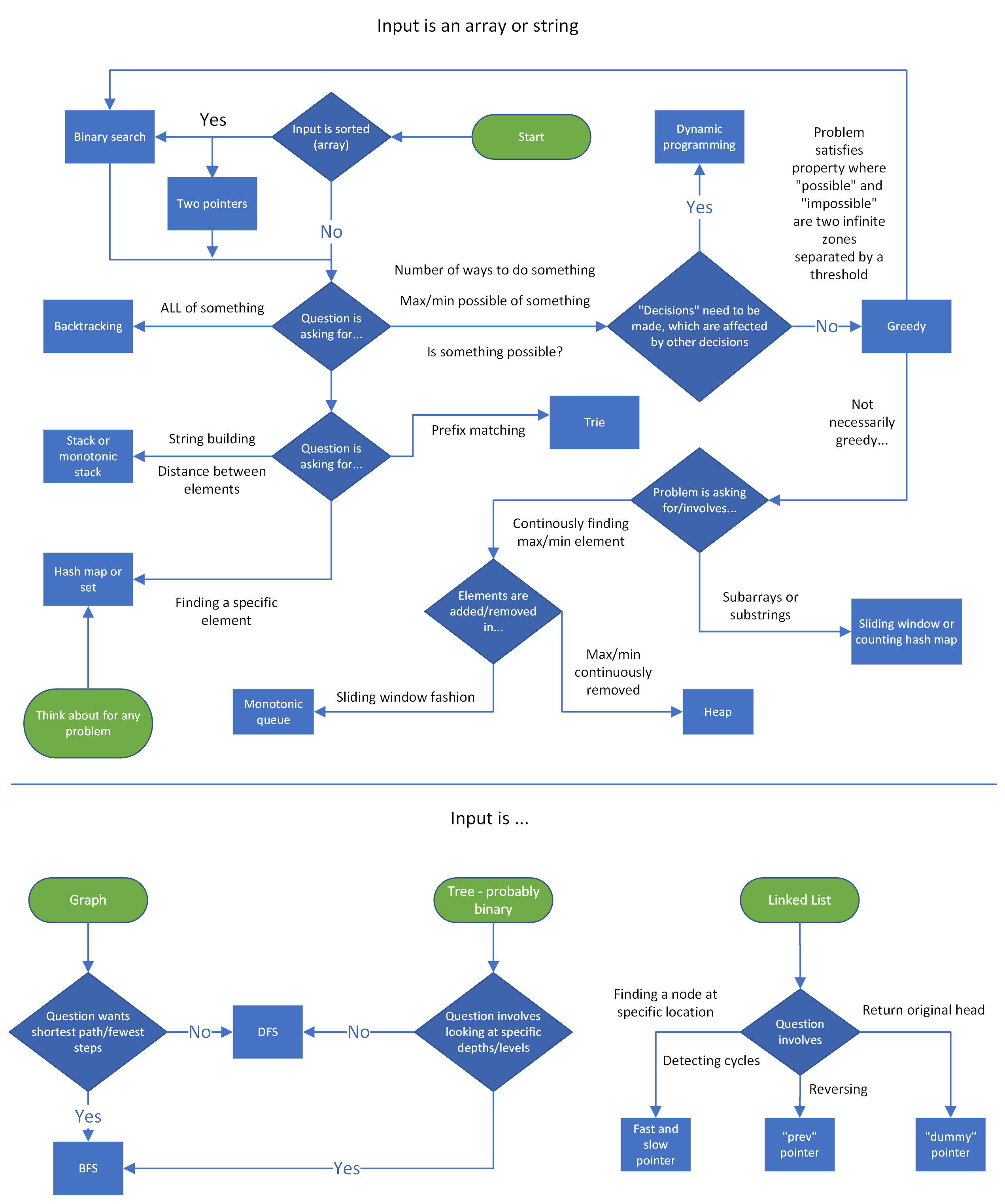
Look at the input and the question asked. Based on that you should be able to detect some pattern. Speak actively with the interviewer and ask questions and seek their confirmation to proceed down particular route. Also think aloud so your interviewer can know what’s going on in your mind. For coding assessment rounds, these patterns should give you a pointer in the right direction.
Pattern Decision Cheatsheet

Code Templates
Two Pointers : one input, opposite ends
def fn(arr):
    left = ans = 0
    right = len(arr) - 1

    while left < right:
        # do some logic here with left and right
        if CONDITION:
            left += 1
        else:
            right -= 1

        # or do both same time: left += 1 and right -= 1

    return ans
This two pointer opposite end inward pattern is useful for comparing elements at opposite ends like valid palindrome or largest container
Two Pointers : two inputs from same direction, exhaust both
def fn(arr1, arr2):
    i = j = ans = 0

    while i < len(arr1) and j < len(arr2):
        # do some logic here
        if CONDITION:
            i += 1
        else:
            j += 1

    while i < len(arr1):
        # do logic
        i += 1

    while j < len(arr2):
        # do logic
        j += 1

    return ans
If you have to compare first element of first array with last element of second array you’re better off reversing the second array and comparing first elements of both arrays.
Unidirectional Traversal
- One pointer finds information and other pointer keeps track of this information.
Staged Traversal
- Both pointers start at same end of the data structure i.e. beginning/end. One pointer is used to search for something, and once found, second pointer finds additional information concerning the first pointer. Things happen in stages.
Sliding Window
def sliding_window(arr):
    left = ans = curr = 0

  "You can use for loop or while loop for right pointer parsing through the array"
  # for right in range(len(arr)):
    while right < len(arr):
        # do logic here to add arr[right] to curr

        while WINDOW_CONDITION_BROKEN:
            # remove arr[left] from curr
            left += 1

        # update ans

        right += 1 # Not needed if using FOR loop

    return ans
Dynamic Sliding Window
- To expand the window advance the right pointer
- To shrink the window advance the left pointer
- To slide the window advance both pointers
Eg. Longest substring with unique characters
Fixed Sliding Window
- Only slide by advancing both pointers. Use when problem asks find a subcomponent of a certain length.
Eg. Substring Anagrams
Prefix Sums / K Sum Subarrays
from collections import defaultdict

def compute_prefix_sums(nums):
    # Start by adding the first number to the prefix sums array.
    prefix_sum = [nums[0]]
    # For all remaining indexes, add 'nums[i]' to the cumulative sum from the previous index.
    for i in range(1, len(nums)):
        # Running total can be a SUM or PRODUCT depends on problem
        running = nums[i] + prefix[-1]
        prefix_sum.append(running)


def compute_k_subarrays(arr, k):
    counts = defaultdict(int)
    counts[0] = 1
    ans = curr = 0

    for num in arr:
        # do logic to change curr
        ans += counts[curr - k]
        counts[curr] += 1

    return ans
There could be +ve or -ve values in the array.
Eg. Sum between range, K-Sum Subarrays, Product Array without Current Element
Linked List : Fast and Slow Pointer
class ListNode:
   def __init__(self, val: int, next: ListNode):
       self.val = val
       self.next = next

def fn(head):
    slow = head
    fast = head
    ans = 0

    while fast and fast.next:
        # do logic
        slow = slow.next
        fast = fast.next.next

    return ans
This is used to detect cycles in a linked list. The distance of fast pointer from slow pointer at every iteration will keep increasing one more step eventually meeting the slow pointer again if there is a cycle.
Reverse Linked List
def fn(head):
    curr = head
    prev = None
    while curr:
        next_node = curr.next
        curr.next = prev
        prev = curr
        curr = next_node

    return prev
When you reverse current node you need to store the next node as temp initially so you can reference it later to continue traversal.
Monotonic Increasing Stack
def monotonic_stack(arr):
    stack = []
    ans = 0

    for num in arr:
        # for monotonic decreasing, just flip the > to <
        while stack and stack[-1] > num:
            # do logic
            stack.pop()
        stack.append(num)

    return ans

def basic_sliding_window(arr):
    left = ans = curr = 0

    for right in range(len(arr)):
        # do logic here to add arr[right] to curr

        while WINDOW_CONDITION_BROKEN:
            # remove arr[left] from curr
            left += 1

        # update ans
    return ans
Monotonic Stack is used to find the break in pattern i.e. pivot point for elements in a stack. This is used to find the largest or smallest index previously.
It’s pattern is similar to a basic sliding window where instead of shifting left pointer based on window condition we just pop elements from the stack till it’s empty or top of the stack is less than or greater than current element depending on our problem.
For loop -> Traverse the array
While loop inside -> Process logic wrt stack / left pointer
Largest Rectange/ Square Area in a Histogram is famous problem for this pattern.
Heap
import heapq

def fn(arr, k):
    heap = []
    for num in arr:
        # do some logic to push onto heap according to problem's criteria
        heapq.heappush(heap, (CRITERIA, num))
        if len(heap) > k:
            heapq.heappop(heap)

    return [num for num in heap]
Min heap : prioritizes smallest element by keeping it at the top
Max heap : prioritizes max element by keeping it at the top
Insertion : O(log(n))
Deletion : O(log(n))
Peek : O(1)
Heapify : O(n)
If you already have an unsorted array you can convert it into a heap in O(n) but adding or removing element will take O(log(n))
A Priority queue is a special type of a heap that allows for customizations in how elements are prioritized.
Finding Median of an Integer Stream or Array is classic heap problem where you maintain a min heap and a max heap with equal or 1 difference values and get the median by popping the top elements in both heaps. Greater values are stored in min heap to get lowest of greater values. Lesser values are stored in max heap to get greatest of lesser values. Their mean is your median if both heaps equal in size.
Binary Tree : DFS Recursive
def dfs(root):
    if not root:
        return

    ans = 0

    # do logic
    dfs(root.left)
    dfs(root.right)
    return ans
Depth first search is usually done recursively for coding rounds. We can reach a null node and check if null and return. No need to look ahead before next recursive call.
Postorder -> Current Node then Left & Right
Preorder -> Left then Right then Current Node. Useful when current node value is derived from it’s children.
Inorder -> Left then Current Node then Right
Think of naming as when to do ordered traversal wrt current node. Post means after current node, pre means before current node.
Binary Tree : DFS Iterative
def dfs(root):
    stack = [root]
    ans = 0

    while stack:
        node = stack.pop()
        # do logic
        if node.left:
            stack.append(node.left)
        if node.right:
            stack.append(node.right)

    return ans
A recursion call creates a stack. If we want to do DFS iteratively then we have to manually initialise and use a stack.
The order of insertion of elements in a stack for preorder or postorder will be as recursive calls made in previous function.
Order of execution for stack is First In Last Out so most recently added nodes will be processed first.
Remember that we first pop the stack to get the current node before adding it’s left and right nodes.
Binary Tree : BFS
from collections import deque

def binary_tree_naive_bfs(root):
    queue = deque([root])
    ans = 0

    while queue:
        current_length = len(queue)
        # do logic naively for nearest
        node = queue.popleft()
        # do logic
        if node.left:
            queue.append(node.left)
        if node.right:
            queue.append(node.right)

    return ans

"Difference here is that we process all elements in a level in one loop hence a for inside while to track state"
def binary_tree_strict_level_bfs(root):
    queue = deque([root])
    ans = 0

    while queue:
        current_length = len(queue)
        # do logic for current level
        # THIS LINE IS DIFFERENCE WITH NAIVE BFS
        for _ in range(current_length):
            node = queue.popleft()
            # do logic
            if node.left:
                queue.append(node.left)
            if node.right:
                queue.append(node.right)

    return ans
This is when we require level order traversal instead of depth order traversal. We explore neighbors then their neighbors and so on.
BFS uses a queue processed in FIFO pattern so that we explore neighbors first level wise.
We fill the queue initially with the first root node.
Based on our requirement for naive or strict level based processing we pop out the elements from the queue and process them and add their children to the queue.
Don’t use BFS for operations that require you find max depth as you’ll end up unnecessarily exploring large parts of the tree/ graph before finding the max depth. Use DFS instead.
Graphs
Graphs are like trees with nodes and edges but there is no strict constraint on their connections.
Any node can be connected to any other node via an edge to form a graph
class GraphNode:
    def __init__(self, val):
        self.val = val
        self.neighbors = []
A node in a graph can have multiple neighbors.
Degree of graph node is number of edges connected to it.
Path is a sequence of nodes connected by edges.
To solve a graph problem we first need to generate an adjacency list or adjacency matrix which we need to use for traversal.

In an adjacency list, the neighbors of each node are stored as a list. Adjacency lists can be implemented using a hash map, where the key represents the node, and its corresponding value represents the list of that node’s neighbors.
In an adjacency matrix, the graph is represented as a 2D matrix where matrix[i][j] indicates an edge between nodes i and j.
Adjacency lists are most common choice as they consume less space especially for sparse graphs.
Adjacency matrices make sense when we handle dense graphs & need to check for existence of edges between two nodes frequently.
Verty important to keep track of visited nodes to prevent infinite loops in cyclic graphs and eliminate double work.
Graph algorithm flowchart :

Graph DFS
#############################################
"For graph node templates we need to traverse the node objects"
class GraphNode:
    def __init__(self, val):
        self.val = val
        self.neighbors = []

def dfs(node: GraphNode, visited: Set[GraphNode]):
    visited.add(node)
    process(node)
    for neighbor in node.neighbors:
        if neighbor not in visited:
            dfs(neighbor, visited)

#############################################

"For the graph templates, assume the nodes are numbered from 0 to n - 1 and the graph is given as an adjacency list."
def recursive_dfs(graph):
    def dfs(node):
        ans = 0
        # do some logic
        for neighbor in graph[node]:
            if neighbor not in seen:
                seen.add(neighbor)
                ans += dfs(neighbor)

        return ans

    seen = {START_NODE}
    return dfs(START_NODE)

def iterative_dfs(graph):
    stack = [START_NODE]
    seen = {START_NODE}
    ans = 0

    while stack:
        node = stack.pop()
        # do some logic
        for neighbor in graph[node]:
            if neighbor not in seen:
                seen.add(neighbor)
                stack.append(neighbor)

    return ans

#############################################
Depending on the problem we have to process the input accordingly.
We can either traverse the graph nodes or convert them to an adjacency list and traverse accordingly.
Graph BFS
from collections import deque

#############################################

"For graph node templates we need to traverse the node objects"
class GraphNode:
    def __init__(self, val):
        self.val = val
        self.neighbors = []

def bfs(node: GraphNode):
    visited = set()
    queue = deque([node])
    while queue:
        node = queue.popleft()
        if node not in visited:
            visited.add(node)
            process(node)
            for neighbor in node.neighbors:
                queue.append(neighbor)

#############################################

"For the graph templates, assume the nodes are numbered from 0 to n - 1 and the graph is given as an adjacency list."
def bfs_adjacency_list(graph):
    queue = deque([START_NODE])
    seen = {START_NODE}
    ans = 0

    while queue:
        node = queue.popleft()
        # do some logic
        for neighbor in graph[node]:
            if neighbor not in seen:
                seen.add(neighbor)
                queue.append(neighbor)

    return ans

#############################################
Same as above when it comes to handling various inputs.
Backtracking
def backtrack(curr, OTHER_ARGUMENTS...):
    if (BASE_CASE):
        # modify the answer
        return

    ans = 0
    for (ITERATE_OVER_INPUT):
        # modify the current state
        ans += backtrack(curr, OTHER_ARGUMENTS...)
        # undo the modification of the current state

    return ans
The code will seem similar to DFS recursive code. This is because recursive DFS is an example of backtracking.
We return once we hit the base case. Till then we iterate through the input / nodes / neighbors / children recursively and get individual answers and combine them into our result and return it to our parent.
State Space Tree
In backtracking, the state space tree, also known as the decision tree, is a conceptual tree constructed by considering every possible decision that can be made at each point in a process.

Here’s a simplified explanation of a state space tree:
- Edges: Each edge represents a possible decision, move, or action.
- Root node: The root node represents the initial state or position before any decisions are made.
- Intermediate nodes: Nodes representing partially completed states or intermediate positions.
- Leaf nodes: The leaf nodes represent complete or invalid solutions.
- Path: A path from the root to any leaf node represents a sequence of decisions that lead to a complete or invalid solution.
Drawing out the state space tree for a problem helps to visualize the entire solution space, and all possible decisions.
Backtracking Algorithm
Traversing the state space tree is typically done using recursive DFS. Let’s discuss how it’s implemented at a high level.
Termination condition: Define the condition that specifies when a path should end. This condition should define when we’ve found a valid and/or invalid solution.
Iterate through decisions: Iterate through every possible decision at the current node, which contains the current state of the problem. For each decision:
- Make that decision and update the current state accordingly.
- Recursively explore all paths that branch from this updated state by calling the DFS function on this state.
- Backtrack by undoing the decision we made and reverting the state.
Below is a crude template for backtracking:
def dfs(state):
    # Termination condition.
    if meets_termination_condition(state):
        process_solution(state)
        return
    # Explore each possible decision that can be made at the current state.
    for decision in possible_decisions(state):
        make_decision(state, decision)
        dfs(state) # USE DFS TO EXPLORE ALL CHILD STATES
        undo_decision(state, decision)  # Backtrack.
There is a lot of redundant work if we reach same state again and again!
Dynamic Programming : Top Down Memoization
def top_down_dp(arr):
    def dp(STATE):
        if BASE_CASE:
            return 0

        if STATE in memo:
            return memo[STATE]

        ans = RECURRENCE_RELATION(STATE)
        memo[STATE] = ans
        return ans

    memo = {}
    return dp(STATE_FOR_WHOLE_INPUT)
Top Down DP is basically Backtracking + Memoization
Explore the states with recurrence relation and cache any intermediate results to avoid double work if you come across the same state again.
Bottom Up DP
def bottom_up_dp(arr):
    # Initialize DP table
    dp = {}  # or array of appropriate size

    # Set base cases
    dp[BASE_STATE] = 0

    # Iterate through states in topological order
    # (from smaller subproblems to larger)
    for STATE in TOPOLOGICAL_ORDER:
        dp[STATE] = RECURRENCE_RELATION(STATE)

    return dp[STATE_FOR_WHOLE_INPUT]
Write a for-loop(s) that iterate over your state variables. If you have multiple state variables, you will need nested for-loops.
Start iterating from the base cases and end at the answer state.
Copy-paste the logic from your function into the for-loop and change the function calls to accessing your array. All dp(…)dp(…) changes into dp[…]dp[…].
Example for Fibonacci Series DP
# Top-down
def fib_top_down(n):
    def dp(i):
        if i <= 1:
            return i
        if i in memo:
            return memo[i]
        memo[i] = dp(i-1) + dp(i-2)
        return memo[i]
    memo = {}
    return dp(n)

# Bottom-up
def fib_bottom_up(n):
    if n <= 1:
        return n
    dp = [0] * (n + 1)
    dp[0], dp[1] = 0, 1  # base cases
    for i in range(2, n + 1):  # topological order
        dp[i] = dp[i-1] + dp[i-2]
    return dp[n]
When to use While loop instead of For loop?
Use while when:
- Step size varies
- Early termination is possible
- Termination condition is complex
- Processing states from a queue/stack
# Variable step sizes
i = 0
while i < n:
    dp[i] = ...
    i += step[i]  # non-uniform jumps

# Early termination
while i < n and not converged:
    dp[i] = ...
    i += 1

# Complex termination conditions
while queue:  # BFS-style DP
    state = queue.pop()
    ...
In practice, 90%+ of bottom-up DP uses for loops because most problems have predictable, sequential state transitions.
Trie
class TrieNode:
    def __init__(self):
        self.children = {}
        self.is_word = False

class Trie:
   def __init__(self):
       self.root = TrieNode()

   def insert(self, word: str) -> None:
       node = self.root
       for c in word:
           # For each character in the word, if it’s not a child of the current node,
           # create a new TrieNode for that character.
           if c not in node.children:
               node.children[c] = TrieNode()
           node = node.children[c] # CHANGE NODE EVERY FOR ITERATION LOOP
       # Mark the last node as the end of a word.
       node.is_word = True

   def search(self, word: str) -> bool:
       node = self.root
       for c in word:
           # For each character in the word, if it’s not a child of the current node,
           # the word doesn't exist in the Trie.
           if c not in node.children:
               return False
           node = node.children[c] # CHANGE NODE EVERY FOR ITERATION LOOP
       # Return whether the current node is marked as the end of the word.
       return node.is_word

   def has_prefix(self, prefix: str) -> bool:
       node = self.root
       for c in prefix:
           if c not in node.children:
               return False
           node = node.children[c] # CHANGE NODE EVERY FOR ITERATION LOOP
       # Once we’ve traversed the nodes corresponding to each character in the
       # prefix, return True.
       return True
We build and use Tries to find String Prefix
We change node in every for loop iteration as you can see in above code to continue searching remainder prefix among children.
All operation be it Insert, Search Word, Search Prefix, Delete take same time complexity of O(n)

Matrix Operation
import copy

def flatten_matrix(matrix):
    # To 1D list
    flat = [elem for row in matrix for elem in row]

    # 1D index to 2D
    row, col = index // cols, index % cols

    # 2D to 1D index
    index = row * cols + col

def copy_matrix(matrix):
    # Shalow copy
    new_matrix = [row[:] for row in matrix]

    # Deep copy
    new_matrix = copy.deepcopy(matrix)

def traverse(matrix, row, col):
    rows, cols = len(matrix), len(matrix[0])

    # Up, Down, Left, Right
    directions = [(-1, 0), (1, 0), (0, -1), (0, 1)]

    # 8 Direction with Diagonals
    directions = [(-1, -1), (-1, 0), (-1, 1),
              (0, -1),           (0, 1),
              (1, -1),  (1, 0),  (1, 1)]
    for dr, dc in directions:
        nr, nc = row + dr, col + dc

        # Boundary check
        if 0 <= nr < rows and 0 <= nc < cols:
            # Process neighbor
            neighbor = matrix[nr][nc]
            # ... do something

def get_row_and_col_elements(matrix, row, col):
    rows, cols = len(matrix), len(matrix[0])

    row_elements = [matrix[row][c] for c in range(cols) if c != col]
    col_elements = [matrix[r][col] for r in range(rows) if r != row]

    return row_elements, col_elements
While traversing a matrix we need to be comfortable with various operations like getting neighbors of a cell, boundary condition check, get all row or column elements of a cell etc.
Dijkstra’s algorithm
from math import inf
import heapq
from collections import defaultdict

edges = [(source, nei_1, w1), (source, nei_2, w2), (source, nei_3, w3)]

graph = defaultdict(list)


# u = source node, v = neighbor node, w = edge distance weight
for u, v, w in edges:
    graph[u].append((v, w))
    graph[v].append((u, w))


distances = [inf] * n
distances[source] = 0
heap = [(0, source)]

while heap:
    curr_dist, node = heappop(heap)

    # THIS PREVENTS MULTIPLE PROCESSING OF VISITED NODES
    if curr_dist > distances[node]:
        continue

    for nei, weight in graph[node]:
        dist = curr_dist + weight
        if dist < distances[nei]:
            distances[nei] = dist
            heappush(heap, (dist, nei))
This algorithm is to find the Shortest Path from source node to each node in the graph if the graph has only non-negative weighted edges.
Initially the distance from source node to all other nodes is infinity.
This is a greedy algorithm where we use a min heap to get closest unvisited nodes. We don’t need to maintain a visited set to prevent double processing. This is because we check current distance from source to the node and skip if it’s more than through intermediate nodes. That way we process it again only if we encounter an even shorter path.
Our greedy assumption is that the closest paths for one node will lead to closest paths for other nodes. That’s why min heap greedy solution to get the nodes with minimum distance first.
Greedy assumption will fail if we have negative edges .